Chapter 6: Short-time Critical Dynamics

6.1  Introduction

A spin model has both static properties (e.g., the critical exponent of the magnetization) and dynamic properties. The latter characterise the behaviour of the system over time, e.g., the manner in which it decays from an initial state of magnetization 1.

This chapter obtains simulation results concerning short-time dynamics in the Ising model and in the 3-state Potts model, compares them with results in the literature, and gives a new result concerning the 4-state Potts model.

Janssen et al. (1989), using a renormalisation group approach, discovered that in the early stages of the relaxation process¹ in an Ising or a q-state Potts model at critical temperature with small initial magnetization one may expect to find (via Monte Carlo studies) an increase in the magnetization before it crosses over to the long-term relaxation behaviour. This initial increase is known as "the critical initial slip" and is characterized by a new universal dynamic critical exponent θ.

Based on the work of Janssen et al. various authors (e.g., Zheng 1998 and Jaster et al. 1999) have noted the following scaling relation for Ising and Potts spin models:

M^(k) (t, τ, L, m₀) = b^-kβ/ν . M^(k) (b^-zt, b^1/ντ, b^-1L, b^x₀.m₀)

where M^(k) is the k-th moment of the magnetization, t is time, τ is the reduced temperature, (T-T_c)/T_c, L is the lattice size, m_o is the initial magnetization, z is the dynamic critical exponent, ν is the critical exponent of the correlation length,²  x_o is a critical exponent called "the scaling dimension of the initial magnetization" and b is a scaling factor.

As shown by Okano et al. 1997 (and in somewhat more detail in Jaster et al. 1999) this has the consequence for the time evolution of the magnetization M(t) in the initial stage of the relaxation process that at the critical temperature M(t) ~ m₀t^θ where θ = (x₀ - β/ν)/z (with β denoting the critical exponent of the magnetization³) is a new universal dynamic critical exponent.

A second consequence is that for zero initial magnetization the 2^nd moment of the magnetization M⁽²⁾(t) ~ t^(d-2β/ν)/z where d is the dimension, β and ν are static critical exponents (as defined above) and z is the dynamic critical exponent.

Thirdly, for zero initial magnetization, the autocorrelation A(t) ~ t^{-d/z + θ} where d, z and θ are as above.

Thus, for a given d, it is possible, by means of a spin model study, to obtain the following (by measuring the slope of log-log plots of the quantity under consideration against time):
(a) An estimate of θ by monitoring the magnetization.
(b) An estimate of z by monitoring the autocorrelation.
(c) An estimate of β/ν by monitoring the 2^nd moment of the magnetization.

In Sections 6.2 and 6.3 we reproduce some measurements for the Ising and the 3-state Potts model given by Okano et al. 1997. Having established that the simulation software gives correct results in these cases we then go on to obtain a new result for θ for the 4-state Potts model and an estimate for z.

6.2  The Ising Model

(i) Magnetization

The magnetization (per spin) in the Ising model is defined as Σ_i(S_i / N) where N is the number of spins and S_i = +1 or -1 for each spin S_i.

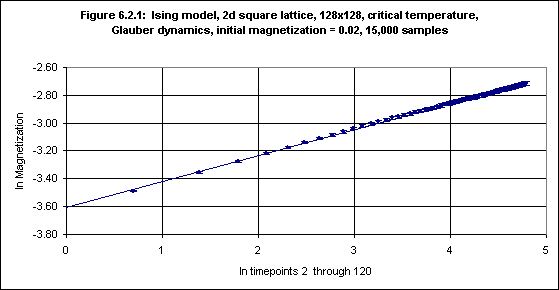
Okano et al. performed simulations using a square lattice of size 128x128 and initial magnetizations, M₀, in the range 0.08 to 0.02 (using both Metropolis and Glauber algorithms). In each case magnetization from timepoints 0 - 120 was measured, and the magnetization against the time was plotted using a log-log plot. Okano et al. were able to obtain a least-squares fit to the data, and the slope of the line gives the value of the short-time dynamic critical exponent θ (for the particular initial magnetization used⁴). Table 1 of Okano et al. (p.736) gives the results for M₀ of 0.08, 0.06, 0.04 and 0.02. By means of reciprocal-size projection Okano et al. then obtained an estimate for M₀ of zero, namely 0.191(1), which is the final estimate for θ for the Ising model (using Glauber dynamics) by Okano et al.

For M₀ = 0.02, Glauber dyamics and 300,000 samples Okano et al. obtained a value of 0.187(1) for θ. This experiment was repeated using the simulation program, with 15,000 samples, and the result (with error bars) is shown in Figure 6.2.1.⁵

The error bars in the logarithm values of the magnetization in Figure 6.2.1 were obtained from the values of the standard deviation of the magnetization as follows, where M = mean magnetization (at a given timepoint) and sd = standard deviation of the measurements of the magnetization (at that timepoint):

Positive error bar: ln(1+sd/M)

Negative error bar: -ln(1-sd/M)

This follows from the algebraic relations:

ln(M+sd) = ln(M) + ln(1+sd/M)

ln(M-sd) = ln(M) - -ln(1-sd/M)

Running the FIT program on the 60 magnetization values, with error bars, yields:⁶

60 data lines read.
Standard deviations present.
Data fitted to y(x) = a + bx.

    a = -3.6129, siga = 0.0042
    b = 0.1888, sigb = 0.0012
chi^2 = 10.6210,    Q = 1.0000

We may conclude that θ for this case is 0.189(1). This is between the value for initial magnetization 0.02 of 0.187(1) obtained by Okano et al. and their final estimate of 0.191(1).

(ii) Autocorrelation

Autocorrelation is a measure of the correlation of the spins of a lattice with their initial state, or more exactly (for the Ising model):

A_Ising(t) = 2.{ Σ_i[δ(S_i,0,S_i,t)] / N } - 1

where N is the number of spins and for the ith spin S_i,0 is its initial value, S_i,t is its value at timepoint t and δ() is the Kronecker delta function: δ(x,y) = 1 if and only if x = y (otherwise 0).⁷  At the initial state the correlation is 1. As spins are flipped the correlation decreases, becoming zero when the spins are totally uncorrelated with their initial state.

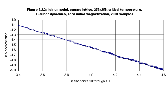
Okano et al. performed a simulation using a square lattice of size 256x256 and zero initial magnetization (using both the Metropolis and the Glauber algorithms and 35,000 samples). The autocorrelation from timepoints 30 - 100 was measured, and plotted against time using a log-log plot. Okano et al. were able to obtain a least-squares fit to the data, and the slope of the line gives the value of -d/z + θ, where d is the dimension (in this case 2) and z is the dynamic critical exponent. With Glauber dynamics Okano et al. obtained a value of -0.737(1) for -d/z + θ.⁸

This experiment was repeated using the simulation program, with 2,800 samples, and the result is shown in Figure 6.2.2 (with error bars).

The error bars in the logarithm values of the autocorrelation in Figure 6.2.2 were obtained from the standard deviation of the autocorrelation as described above.

Running the FIT program on the autocorrelation log values, with error bars, yields:

71 data lines read.
Standard deviations present.
Data fitted to y(x) = a + bx.

    a = -1.5956, siga = 0.0091
    b = -0.7391, sigb = 0.0023
chi^2 = 39.4005,    Q = 0.9984

From this we may conclude that -d/z + θ is -0.739(2), which is almost the same as the -0.737(1) obtained by Okano et al.

(iii) Second Moment of the Magnetization

In the Ising model the 2^nd moment of the magnetization, M⁽²⁾, is simply the mean square magnetization (or rather, for a given timepoint t, the mean of the squares of the magnetizations measured at t averaged over many samples), i.e.,

M⁽²⁾ = [ (Σ_iS_i) / N ]²

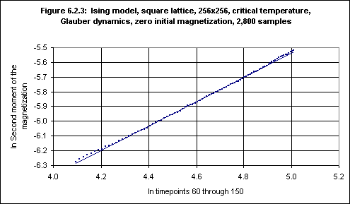
In the simulation performed by Okano et al. to measure the autocorrelation the 2^nd moment of the magnetization was also measured, over timepoints 60 - 150. After plotting M⁽²⁾ against time using a log-log plot Okano et al. obtained a least-squares fit to the data, and the slope of the line gave the value of (d-2β/ν)/z, where β is the critical exponent of the magnetization and ν is the critical exponent of the correlation length. With Glauber dynamics Okano et al. obtained a value of 0.817(7) for (d-2β/ν)/z.

In the same repetition, using the simulation software, of the experiment in which the autocorrelation was measured the 2^nd moment of the magnetization was also measured, and the result is shown in Figure 6.2.3.⁹

Running the FIT program on the ln M⁽²⁾ values yields:

91 data lines read.
Standard deviations absent.
Data fitted to y(x) = a + bx.

    a = -9.6546, siga = 0.0112
    b = +0.8234, sigb = 0.0024
chi^2 = 0.0032

From this we may conclude that (d-2β/ν)/z is 0.823(3), which is consistent with the value of 0.817(7) obtained by Okano et al.

6.3  The 3-state Potts Model

(i) Magnetization

For the q-state Potts model magnetization (per spin) is defined as follows:

M = { q / [(q-1).N] } . Σ_i[ δ(S_i,1) - 1/q ]

where δ(S_i,1), the Kronecker delta, is 1 if S_i = 1 and 0 otherwise.¹⁰ Thus if all spins have spin value +1 then M = 1, if all have a spin value other than +1 then M = -1/(q-1), and if the spin values 1, ..., q are distributed randomly among the N spins (so that N/q have spin value +1) then M = 0.

Okano et al. performed simulations with the 3-state Potts model similar to those described in the previous section. To measure the value of the short-time dynamic critical exponent θ a square lattice of linear size 72 and initial magnetizations, M₀, in the range 0.08 to 0.02 (using both the Metropolis and the Glauber algorithms) were used.

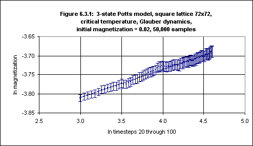
Table 3 of Okano et al. 1997 (p.741) gives the results for M₀ of 0.08, 0.06, 0.04 and 0.02. By means of reciprocal-size projection Okano et al. then obtained an estimate for M₀ = 0, namely 0.075(3), which is the final estimate for θ for the 3-state Potts model given by Okano et al.¹¹

For M₀ = 0.02, Glauber dyamics and 600,000 samples Okano et al. obtained a value of 0.084(3) for θ. This experiment was repeated using the simulation program, with 50,000 samples, and the result (with error bars) is shown in Figure 6.3.1.

Running the FIT program on the magnetization log values (for timepoints 20 through 100, the same as used by Okano et al.) with error bars yields:

81 data lines read.
Standard deviations present.
Data fitted to y(x) = a + bx.

    a = -4.0331, siga = 0.0114
    b = +0.0742, sigb = 0.0029
chi^2 = 5.8651,    Q = 1.0000

From this we may conclude that θ for this case is 0.074(3). This is lower than the value 0.084(3) for initial magnetization of 0.02 obtained by Okano et al. but is close to their final estimate for the square 3-state Potts θ of 0.075(3).¹²

(ii) Autocorrelation

The definition of autocorrelation for the q-state Potts model is:

A_Potts(t) = { Σ_i[ δ(S_i,0,S_i,t) - 1/q ] } / N

that is,

A_Potts(t) = ( { Σ_i[ δ(S_i,0,S_i,t) ] } / N ) - 1/q

At the initial state the correlation is (q-1)/q. As spins are flipped over time the correlation decreases, becoming zero when the spins are totally uncorrelated with their initial state.¹³

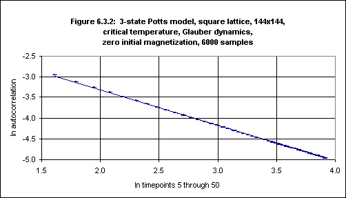
Okano et al. performed simulations with square lattices of size 144, 288 and 576 and zero M₀ (using both the Metropolis and the Glauber algorithms¹⁴). The autocorrelation over the first 85 timepoints was measured. Okano et al. plotted autocorrelation against time for timepoints 5 - 50 using a log-log plot and averaged the values of the slopes of the plots for the three lattice sizes to obtain a value for -d/z + θ of -0.836(2).¹⁵

For lattice size 144 Okano et al. obtained -0.839(1) for -d/z + θ. This experiment was repeated using the simulation program, with 6000 samples, and the result is shown in Figure 6.3.2 (with error bars).

Running the FIT program on the autocorrelation log values, with error bars, yields:

46 data lines read.
Standard deviations present.
Data fitted to y(x) = a + bx.

    a = -1.5643, siga = 0.0012
    b = -0.8714, sigb = 0.0005
chi^2 = 914.9231,    Q = 0.0000

From this we might conclude that -d/z + θ is -0.871(1). However, the Q value is zero, so (following Press et al., 1992, p.664, quoted in Appendix 4) we must question this result. The problem appears to come from choosing a range of timepoints (namely, 5 - 50) which begins too early. Okano et al. write:

Even though universal behaviour is expected in the macroscopic early time, in general, the dynamic system needs a certain microscopic time period to get rid of the microscopic short-wave effects and to enter the macroscopic quasi-stable state. Such a time period is called the microscopic time scale t_mic. It is only for t > t_mic that the exponents extracted from the short-time dynamics will be universal, i.e. will be independent of the algorithms and other microscopic details. (Okano et al., 1997, p.728).

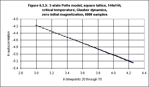
If we do a log-log plot of autocorrelation against time for timepoints 20 - 70, rather than 5 - 50, we obtain Figure 6.3.3 (with error bars):

Running the FIT program on the autocorrelation log values, with error bars, yields:

51 data lines read.
Standard deviations present.
Data fitted to y(x) = a + bx.

    a = -1.6582, siga = 0.0061
    b = -0.8417, sigb = 0.0017
chi^2 = 30.9428,    Q = 0.9795

Now Q > 0.1 and we may conclude that -d/z + θ is -0.842(2). This is consistent with the result for the lattice of size 144 of -0.839(1) obtained by Okano et al.

(iii) Second Moment of the Magnetization

Following the definition given by Okano et al. 1997 (p.743) of the 2^nd moment of the magnetization, M⁽²⁾, for the 3-state Potts model we define M⁽²⁾ for the q-state Potts model as:

M⁽²⁾ = { q / [(q-1).N] }² . [ ( Σ_r { Σ_i[δ(S_i,r) - 1/q] }² ) / q ]

where for 1 ≤ r ≤ q, δ(S_i,r) is 1 if S_i = r and 0 otherwise.

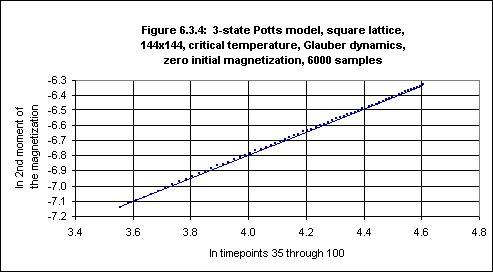
In the simulation performed by Okano et al. to measure the autocorrelation, M⁽²⁾ was also measured, over timepoints 35 - 100. After plotting M⁽²⁾ against time using a log-log plot Okano et al. obtained a least-squares fit to the data, and the slope of the line gave the value of (d-2β/ν)/z, where β and ν are as before. Okano et al. averaged over lattice sizes 144 and 288, using Glauber dynamics, to obtain a value of 0.788(1) for (d-2β/ν)/z (see Okano et al. 1997, Table 5, p.745). For lattice size 144 Okano et al. obtained a value of 0.789(2).

In the repetition, with the simulation software, of the experiment in which the autocorrelation was measured (using 6000 samples and a lattice of size 144) M⁽²⁾ was also measured; the result is shown in Figure 6.3.4.¹⁶

Running the FIT program on the ln M⁽²⁾ values yields:

66 data lines read.
Standard deviations absent.
Data fitted to y(x) = a + bx.

    a = -9.8497, siga = 0.0046
    b = +0.7644, sigb = 0.0011
chi^2 = 0.0005

from which we may conclude that (d-2β/ν)/z is 0.764(1), which is smaller than the value of 0.789(2) obtained by Okano et al.

The value one obtains for (d-2β/ν)/z depends on the range of timepoints. By fitting a line to the ln M⁽²⁾ values over timepoints 20 - 60 one obtains:

41 data lines read.
Standard deviations absent.
Data fitted to y(x) = a + bx.

    a = -9.9446, siga = 0.0061
    b = +0.7890, sigb = 0.0017
chi^2 = 0.0004

from which one could also conclude that (d-2β/ν)/z is 0.789(2), which is the same as the value obtained by Okano et al.

The results from the simulation program which have been described in Sections 6.2 and 6.3 for the Ising model and the 3-state Potts model on a square lattice, when compared to the results obtained by Okano et al., show that we are justified in having some degree of confidence in the simulation program. We may thus proceed to apply it to the case of the 4-state Potts model.

6.4  The 4-state Potts Model

Simulations were performed using Glauber dynamics over the first 100 timepoints for the pure 4-state Potts model using a square lattice, with sizes of 16, 32 and 64, and initial magnetizations, M₀, of 0.08, 0.06, 0.04, 0.02, and zero. The magnetization was measured for M₀ = 0.08 to 0.02, and the autocorrelation was measured for M₀ = 0. For lattice sizes 16 and 32, 250,000 samples were used, and for lattice size 64, 100,000 samples. The average time for simulations (on a 330 MHz Intel PC) was 6, 22 and 33 hours for lattice sizes 16, 32 and 64 respectively, and the total computing time was 305 hours (12.7 days).

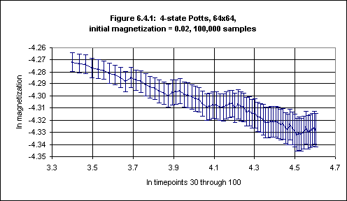
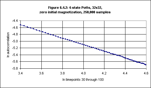
Figures 6.4.1 and 6.4.2 (based on data in Tables 6.4.1 and 6.4.2 in Appendix 5) are examples of data from simulations with a particular size and initial magnetization, and show log-log plots against time (timepoints 30 through 100) for a square lattice of (a) the magnetization (with lattice size 64, initial magnetization 0.02 and 100,000 samples) and (b) the autocorrelation (with lattice size 32, zero initial magnetization and 250,000 samples).

The error bars in the logarithm values of the magnetization in Figure 6.4.1 were obtained as in Section 6.2(i).

Running the FIT program on the log values of the magnetization over timepoints 30 - 100 gives:

71 data lines read.
Standard deviations present.
Data fitted to y(x) = a + bx.

    a = -4.1058, siga = 0.0157
    b = -0.0490, sigb = 0.0039
chi^2 = 2.5558,    Q = 1.0000

Thus the slope of the least-squares fit in this case (a first approximation to the 4-state Potts θ) is -0.0490(39), or rather -0.049(4).

The error bars in the logarithm values of the autocorrelation values in Figure 6.4.2 were obtained from the values of the standard deviation of the autocorrelation as follows, where A = autocorrelation (at a given timepoint) and sdA = standard deviation of the autocorrelation (at that timepoint):

Positive error bar: ln(1+sdA/A)

Negative error bar: -ln(1-sdA/A)

Running the FIT program on the log values of the autocorrelation over timepoints 30 - 100 gives:¹⁷

71 data lines read.
Standard deviations present.
Data fitted to y(x) = a + bx.

    a = -1.2223, siga = 0.0067
    b = -0.9705, sigb = 0.0017
chi^2 = 38.2004,    Q = 0.9990

Thus the slope of the least-squares fit in this case (a first approximation to -d/z + θ) is -0.9705(17).

The strategy here adopted is as follows:

(i) An estimate for the 4-state Potts θ will be arrived at by measuring, for each of the three lattice sizes 16, 32 and 64, the slope of the log-log plot of magnetization values over timepoints 30 - 100 for initial magnetizations, M₀, of 0.08, 0.06, 0.04 and 0.02, and projecting the slopes to M₀ = 0, then projecting these values to 1/size = 0.
(ii) An estimate for -d/z + θ will be arrived at by measuring, for each lattice size, with M₀ = 0, the slope of the log-log plot of autocorrelation values over timepoints 30 - 100 and projecting to 1/size = 0.
(iii) From (i) and (ii) we hope to obtain the 4-state Potts dynamic critical exponent, z.

(i) Magnetization

As noted in Section 6.1, M(t) ~ m₀t^θ, where θ is the exponent of the critical initial slip, which is thus measured by the slope of a log-log plot of magnetization against time (after discarding a number of initial timepoints).

The magnetization over the first 100 timesteps in the 4-state Potts square lattice was measured for initial magnetizations of 0.08 to 0.02. The slopes of the least-squares fit to the log values of the magnetization data against timepoints 30 - 100 in each of these twelve cases (three lattice sizes and four initial magnetizations) were obtained by the use of the 4STPFIT program written by the author to analyse the data from these 4-state Potts simulations. This program is described in Appendix 4, "The FIT Programs", with two examples of results, namely, those obtained by running the program on the data (a) for lattice size 64 and M₀ = 0.02 and (b) for lattice size 32 and M₀ = 0 (which are the examples graphed above).

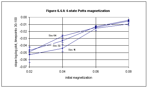
The slopes of the log-log plots of magnetization against time (for timepoints 30 through 100) are given in Table 6.4.4 and are shown in Figure 6.4.4.

Table 6.4.4
4-state Potts, short-time dynamics
Slope of magnetization (timepoints 30-100)
Initial magnetization	0.08	0.06	0.04	0.02
Slope
16	-0.0093	-0.0155	-0.0438	-0.0530
32	-0.0040	-0.0132	-0.0334	-0.0468
64	-0.0052	-0.0141	-0.0270	-0.0490
Errors
16	0.0024	0.0033	0.0050	0.0107
32	0.0012	0.0016	0.0024	0.0050
64	0.0009	0.0012	0.0019	0.0039
Q
16	1.0000	1.0000	1.0000	1.0000
32	1.0000	1.0000	1.0000	1.0000
64	1.0000	1.0000	1.0000	1.0000

The FIT program was then used on the data for each of the lattice sizes 16, 32 and 64 to obtain a least-squares fit and so to project the values to M₀ = 0, to obtain the following (the input data is displayed if the /data command-line parameter is used):

Lattice size 16:

0.08, -0.0093, 0.0024
0.06, -0.0155, 0.0033
0.04, -0.0438, 0.0050
0.02, -0.0530, 0.0107

    a = -0.0660, siga = 0.0076
    b = +0.7308, sigb = 0.1103
chi^2 = 6.6040,    Q = 0.0368

Lattice size 32:

0.08, -0.0040, 0.0012
0.06, -0.0132, 0.0016
0.04, -0.0334, 0.0024
0.02, -0.0468, 0.0050

    a = -0.0579, siga = 0.0037
    b = +0.6866, sigb = 0.0533
chi^2 = 7.3314,    Q = 0.0256

Lattice size 64:

0.08, -0.0052, 0.0009
0.06, -0.0141, 0.0012
0.04, -0.0270, 0.0019
0.02, -0.0490, 0.0039

    a = -0.0513, siga = 0.0028
    b = +0.5864, sigb = 0.0412
chi^2 = 9.6777,    Q = 0.0079

Summarizing, we obtain:

Table 6.4.5
Size	1/size	Proj. zero	Error	Q
16	0.062500	-0.0660	0.0076	0.0368
32	0.031250	-0.0579	0.0037	0.0256
64	0.015625	-0.0513	0.0028	0.0079

We can now plot the projected slopes for M₀ = 0 against the reciprocal of the lattice size to obtain the slope for M₀ in the ideal case of the infinite lattice:

0.0625,   -0.0660, 0.0076
0.03125,  -0.0579, 0.0037
0.015625, -0.0513, 0.0028

    a = -0.0464, siga = 0.0045
    b = -0.3352, sigb = 0.1614
chi^2 = 0.1225,    Q = 0.7263

Thus we arrive at an estimate for the 4-state Potts θ of -0.046(5). Okano et al. 1997 (p.745) remark that "not all the models will have a positive θ. For example, for the Potts model with q = 4 the exponent θ is likely negative or very close to zero." This result confirms that expectation.

(ii) Autocorrelation

As noted in Section 6.1, A(t) ~ t^{-d/z + θ}, where θ is as above, d is the dimensionality (in this case 2) and z is the dynamic critical exponent. Thus by measuring the slope of a log-log plot of autocorrelation against time (after discarding a number of initial timepoints) we can obtain z if we know θ.

The autocorrelation was measured for M₀ = 0. The slopes of the least-squares fits to the log values of the autocorrelation data against timepoints 30 - 100 for each of the lattice sizes were obtained by the use of the 4STPFIT program (described in Appendix 4) and are given in Table 6.4.6.

Table 6.4.6: Autocorrelation (zero initial magnetization)
Size	1/size	Slope A	Error	Q
16	0.062500	-1.0337	0.0032	0.9931
32	0.031250	-0.9705	0.0017	0.9991
64	0.015625	-0.9706	0.0011	0.7991

We can now plot the autocorrelation slopes for M₀ = 0 against the reciprocal of the lattice size to obtain the slope in the ideal case of the infinite lattice:

0.0625,   -1.0337, 0.0032
0.03125,  -0.9705, 0.0017
0.015625, -0.9706, 0.0011

    a = -0.9499, siga = 0.0018
    b = -1.0887, sigb = 0.0673
chi^2 = 97.8233,    Q = 0.0000

Unfortunately the Q-value is zero, a sign that something is not right.

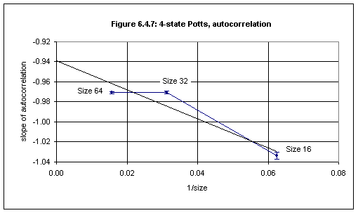
Figure 6.4.7 shows the plot for the slopes of A for each of the sizes 16, 32 and 64.

The reason for the zero Q-value seems to be that the errors have been underestimated.¹⁸  We can calculate a least-squares fit without reference to the error bars, obtaining (with the use of the FIT program):

0.0625,   -1.0337
0.03125,  -0.9705
0.015625, -0.9706

    a = -0.9390, siga = 0.0208
    b = -1.4427, sigb = 0.5020
chi^2 = 0.0003

thus taking -0.939(21) as our estimate for -d/z + θ.¹⁹

(iii) The dynamic critical exponent z

Let slopeA = -d/z + θ, then since d = 2 we have z = 2/(θ - slopeA). In section (i) we arrived at a value of -0.046(5) for θ, so by using the value obtained for slopeA in section (ii) we arrive at an estimate of z, namely 2.240(67), or 2.24(7).

The errors are obtained by noting the extreme values for 2/(θ - slopeA) based on the errors for slopeA and for θ.

Okano et al. (1997) obtained z = 2.155(3) for the Ising model and 2.196(8) for the 3-state Potts model. For the 3-state Potts model Arcangelis and Jan (1986) obtained 2.43(15), and Schülke and Zheng (1995) obtained z = 2.198(8).

Only two published values for the 4-state Potts z were found in the literature, neither of them recent. Arcangelis and Jan (1986) obtained 2.36(20) using a dynamic Monte Carlo renormalization group method, and Jain (1987) obtained 2.94(29) based on Monte Carlo simulations on the square lattice. Both of these are probably too large.

If there were a linear relation between q and z for the q-state Potts model then our estimate of 2.24(7) for the 4-state Potts z would be consistent with it because the FIT program tells us that the following least squares fit gives a Q-value of 0.9884:²⁰

2, 2.155, 0.003
3, 2.197, 0.008
4, 2.240, 0.067

    a = +2.0709, siga = 0.0179
    b = +0.0420, sigb = 0.0083
chi^2 = 0.0002,    Q = 0.9884

Title page

Contents

Next: Chapter 7

References