Chapter 2: The Simulation Program and its Validation

Chapter 2: The Simulation Program and its Validation
2.1 The Simulation Program¹

The simulation program (ISM.EXE), which is written in C, is designed to construct in computer memory an Ising or a q-state Potts spin model of a specified type and to run that model (with a specified dynamics algorithm and lattice geometry, using periodic boundary conditions) so as to simulate a system of magnetic spins evolving over time.² In accord with the aims of computational physics as discussed in Section 1.2, the spin model is studied to attain knowledge of real physical systems which are believed to have an analogous structure and functioning.

Good simulation software relies on a good source of random numbers. It is impractical to use a truly random source based on a physical process (e.g., radioactive decay) so a source based upon a deterministic computational source is used. Beginning with some "seed" integer a sequence of positive integers is generated; these can be converted to numbers between 0 and 1. The generator should have the following properties:

Reproducibility (a given seed number always produces the same sequence of random numbers, so simulations can be repeated exactly if desired).

Efficiency (very little computer memory and very little computation time are required to produce the next number in the sequence, since a simulation usually requires the generation of many millions of random numbers).

Long period (any sequence of random numbers should continue for a long time without repeating itself).

Independence and unpredictability (if the seed number is not known then there should be no way to predict the continuation of a sequence of random numbers based on knowledge of the particular numbers generated up to that point).

Uniform distribution (the random numbers, whether integers or numbers between 0 and 1, should be uniformly distributed over the range of possible numbers).

The presence of properties (iv) and (v) can be tested by the application of statistical tests, which look for regularities or anomalies in the random number sequence.

The random number generator used in this simulation program generates random numbers at a speed of 3.39 million per second (on a 330 Mhz PC), and has a period of more than 10¹⁸. It is discussed in detail in Appendix 2, "The Random Number Generator", where the results of a chi-square test are given.

Running the simulation program with no command line arguments gives:

Syntax: ISM.EXE input_file_1.IN [input_file_2.IN [...]] Output data file has same name with extension .OUT. For the format of the input data use: ISM.EXE /F

The parameters for a simulation are specified in an input file, and several simulations may be run in succession by including several input file names on the command line. The simulation program has been written to handle a variety of models, lattice geometries, types of dilution, etc. The program provides a summary of the input parameters if it is run with the command line: ISM /F, as follows:

------------ ISM V1.93 INPUT PARAMETERS (SPIN MODEL DYNAMICS) ------------ Parameter name Permitted values lattice type: SQU | HON | TRI | CUB | DIA | HC4 lattice size: 4 - 4096 (2d), 4 - 256 (3d), 4 - 64 (4d) model: Is[ing] | q-[state Potts] q-value: 2 - 15 // q-state Potts model only dynamics: ME[tropolis] | GL[auber] | SW[endsen-Wang] | WO[lff] temperature: 0.001 - 50.000 // or "critical" temperatures: // Separate multiple temperatures with commas initial magnetization: -1.0 - +1.0 // >= -1/(q-1) for q-state Potts site concentration: 0.001 - 1.000 bond concentration: 0.001 - 1.000 number of configurations: 1 - 100,000 // 1 for a non-diluted lattice number of spin assignments: 1 - 100,000 number of repetitions: 1 - 500 // Using different random numbers number of timeslices: 2 - 10,001 step length: 1 - 10,000 // timesteps between timeslices percentage range for mean: 1 - 100 Use "Y[es]" or "N[o]" for the following (1st three required): precompute nn sites: absolute magnetization: timeslice values: second moment: autocorrelation: map file: internal energy: Binder cumulant: log values: adjust zero initial magnetization:

Or in other words:

Lattice type: Square, honeycomb, triangular, cubic, diamond, hypercubic

Lattice size: Maximum lattice size depends on dimensionality and dynamics algorithm (smaller with cluster algorithms).

Model: Ising or q-state Potts (for q in the range 2 through 15).

Dynamics: Metropolis, Glauber, Swendsen-Wang or Wolff.

Once the type of lattice is specified, the initial state of the system is defined as follows:

Temperature(s): 0.0 – 20.0. The temperature can also be specified as "critical", in which case the critical temperature for the type of spin system is used, if known. Multiple temperatures are accepted.

Initial magnetization: –1.0 through +1.0 (Initial magnetization must be ≥ –1/(q–1) for the q-state Potts model.)

Site concentration: 0.001 – 1.0 (the concentration of occupied sites).

Bond concentration: 0.001 – 1.0 (the concentration of open bonds among pairs of spins located on nearest neighbour sites).

For a pure lattice both concentrations are specified as 1.0 (the default value). It is possible to simulate a system which is simultaneously both site- and bond-diluted.

Normally the program performs many simulation runs. Each such run is termed a "sample". It is desirable to distribute these samples over a range of possible initial configurations. In the case of a site-diluted (resp. bond-diluted) lattice, with a certain concentration of sites (resp. bonds), the occupied sites (resp. open bonds) may be varied, giving different configurations. Given a particular configuration of occupied sites and open bonds the manner of assigning spin values to the spins (on occupied sites) may be varied, giving different spin assignments. Given a particular configuration and a particular assignment of spin values, a run may be repeated with different random numbers, giving different repetitions. The program allows:

Number of configurations: 1 – 100,000 (but only 1 for a non-diluted lattice)

Number of spin assignments: 1 – 100,000

Number of repetitions: 1 – 500

The simulation program allows four forms of dynamics: Metropolis, Glauber, Swendsen-Wang and Wolff. Each form of dynamics is a method for updating the spins in the spin model. In the first two methods spins are updated individually, and in the second two methods they are updated in clusters. In all four methods, however, the equilibration process may be divided into "timesteps" and "timepoints".

A timestep is one "sweep" through the lattice, in which each spin is considered (for possible change) once and once only.³ The number of timesteps is, in other terminology, the number of "Monte Carlo steps per spin". A "timepoint" is a state of the model after n timesteps (n ≥ 0).

Timepoints are analogous to points in time, and the change in the state of the spin model is analogous to the temporal evolution of the system being modelled.

A "timeslice" is a timestep at which measurements are carried out. Three quantities are measured: (i) the magnetization per spin (optionally, the absolute value thereof), (ii) the actual internal energy of the spin system and (ii) the autocorrelation. The first timeslice is the initial timepoint. Measurements are then taken after every n timesteps, for n ≥ 1, for as many timesteps as were requested.

The results that the simulation program prints are averages at each timeslice over a (possibly large) number of samples (where a "sample" is one run of the requested number of timesteps starting from some spin assignment and, in the case of a dilute lattice, from some configuration of occupied sites).

Two of the input parameters used by the simulation program are "number of timeslices" and "step length". The step length is the number n of timesteps between timeslices. The number of timeslices, including the initial state, can range from 11 to 10,001, and the step length can range from 1 to 10,000.

The simulation program also takes as input parameters whether or not to calculate the following four quantities: the internal energy per spin, the standard deviation of the magnetization, the second moment of the magnetization, the autocorrelation and the Binder cumulant. If internal energy is measured then results for specific heat per spin are given also. In the remainder of this section we will assume that all quantities are to be measured.

Magnetization per spin is a quantity dependent on the values of the spins in a particular state of the spin model. It is always a value between +1 and -1. It is derived from the values of the spins. The derivation of this value from the actual number of spins in various states depends on the model (Ising or q-state Potts).

At each timeslice during a given run the magnetization (per spin) of the spin system is monitored, and the value is added to a running total (which, of course, begins at zero). A running total is also kept of the square of the magnetization (per spin), and the fourth power thereof, at each timeslice.

A running total is kept of the autocorrelation value, which is also calculated differently in the two kinds of spin model.

For each timeslice a running total is kept of the actual internal energy of the spin system (not the internal energy per spin) and the square of this quantity. The internal energy, like the magnetization, depends on the values of the spins (and also on the spins in the immediate neighbourhood of a spin) and is calculated differently for the Ising and the q-state Potts models.

After all runs are completed we have, for each timeslice, six numbers, as follows, where n >= 0 denotes the timeslice number:

m(n) sum of the magnetization (per spin) values

m²(n) sum of the squares of the magnetization values

m⁴(n) sum of the fourth powers of the magnetization values

a(n) sum of the autocorrelation values

e(n) sum of the actual internal energy values

e²(n) sum of the squares of the internal energy values

Analysis, resulting in the values printed in the report (indicated below by italics), is then performed as follows, where N is the number of samples:

For each timeslice n:

The mean magnetization (per spin) = M = m(n) / N.
The mean square magnetization = M⁽²⁾ = m²(n) / N
The standard deviation of the magnetization is then (assuming N > 1) given by √ [ ( M⁽²⁾ - M² ) / ( N - 1 ) ]
The second moment of the magnetization is, in the case of the Ising model, the same as the mean square magnetization. In the case of the Potts model it is calculated in a more complex manner.⁴
The Binder cumulant = 1 - [ m⁴(n) / N ] / [ 3.(M⁽²⁾)² ].
The mean autocorrelation = a(n) / N.
The mean actual internal energy = U = e(n) / N.
The internal energy per spin is the mean actual internal energy divided by the number of spins in the spin system.
The mean square of the actual internal energy = U⁽²⁾ = e²(n) / N.
The actual specific heat = ( U⁽²⁾ - U² ) / T², where T denotes temperature.
The specific heat per spin is this divided by the number of spins in the spin system.

Percentage range for mean: 1 - 100

When a quantity such as the magnetization or the Binder cumulant is measured the value given is an average over a range of timepoints occurring after the system has reached equilibrium (i.e., a time average). E.g., if (using Wolff dynamics) it is known by observeration that measurements of quantities in a particular system stabilize after 30 timesteps, and measurements are made over 100 timesteps, then one might specify percentage range for mean as 40, meaning that the final value for the quantities measured is an average over timepoints 60 through 100.

Some input parameters have Yes or No values, in particular: Absolute magnetization, Timeslice values and Precompute nn sites.

If absolute magnetization is Yes then the absolute value of the magnetization is measured. This is necessary when Swendsen-Wang or Wolff dynamics are used, since in these cases the magnetization often flips between positive and negative within a few timesteps.

If timeslice values is Yes then the values of the quantities measured are reported for each timeslice (otherwise only the final time averages are reported).

If precompute nn sites is set to No then the locations of nearest neighbour sites are repeatedly calculated for many spin updates, which requires a significant amount of computer time. However if precompute nn sites is set toYes then the locations of the nearest neighbours of all sites are precomputed, stored in a large array and retrieved as required. This increases significantly the amount of memory required and is helpful only if the additional memory used does not cause memory to be swapped out to disk (which requires much more time than repeated computation of nearest neighbour locations).

Before using the simulation program to obtain data as the basis of new research it is necessary to ensure that the program works correctly, that is, that it is a valid implementation of the Ising and the q-state Potts spin models. This has been done here by reproducing some known results, details of which are given in the remainder of this chapter.

Appendix 3 contains information about several input files for the simulation program which are given on the accompanying computer disk. These specify some of the many simulations carried out during the course of this work. The output obtained from these simulations is displayed in various graphs in later sections, and may be reproduced by running the program with the supplied input files (although due to random variations and sometimes small numbers of samples such simulations will not reproduce the reported results exactly).

2.2 Comparison of Results for Internal Energy and Specific Heat with Those from High Temperature Series Expansion

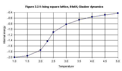
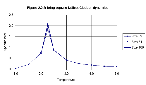
Simulations were performed for the pure Ising square model for T = 1.0 to 5.0 in steps of 0.5 (plus the critical temperature, T ≅ 2.269). The internal energy per spin and the specific heat per spin were measured.5

Lattice sizes of 32x32, 64x64 and 100x100 were used, with the number of samples ranging from 1000 to 8000. Figure 2.2.1 shows a plot of internal energy per spin against temperature (the internal energy per spin approaches zero asymptoticly) for lattice size 64x64. (The values of the internal energy for the other lattice sizes are almost the same.) Figure 2.2.2 shows a plot of specific heat per spin against temperature for the three lattice sizes. The data for these plots is given in Table 2.2.1 in Appendix 5.⁶

Error bars were not calculated. The point of the simulations in this section were not so much to establish results concerning internal energy and specific heat as such but rather to ascertain whether the simulation software gives results in accord with high temperature series expansions (which, of course, have no error estimates associated with them).

The method of high temperature series expansions (described in Yeomans 1992) leads to a formula for the free energy for temperatures higher than the critical temperature. From this can be derived formulae for the internal energy and the specific heat.

Yeomans (1992, p.83) gives the following expression for the free energy of a spin system with N spins at temperature T :

F = -Nk_BT ( ln2 + v² + 3/2 v⁴ + 7/3 v⁶ + 19/4 v⁸ + 61/5 v¹⁰ + …)

where k_B is Boltzman's constant, v = tanh(βJ) and β = 1/(k_BT). It is usual to put J = k_B = 1.

We may obtain the internal energy U by differentiating this with respect to β. So doing, we obtain the following formula for the internal energy per spin:

U/N = -2k sech²(1/T) ( a₂.v + 2.a₄.v³ + 3.a₆.v⁵ + 4.a₈.v⁷ + 5.a₁₀.v⁹ + …)

where a₂= 1, a₄= 3/2, a₆= 7/3, a₈= 19/4 and a₁₀= 61/5.

We may obtain the specific heat C by differentiating this with respect to T. So doing, we obtain the following formula for the specific heat per spin:

C/N = (2k/T²) [ sech⁴(1/T) ( 1 + 3.b₃.v² + 5.b₅.v⁴ + 7.b₇.v⁶ + 9.b₉.v⁸ + …)
- 2 sech²(v) tanh(v) ( v + b₃.v³ + b₅.v⁵ + b₇.v⁷ + b₉.v⁹ + …) ]

where b₃ = 3, b₅ = 7, b₇ = 19 and b₉ = 61.

Values for the internal energy and the specific heat for T = 3.0, 3.5, 4.0, 4.5 and 5.0 were obtained from these formulae for comparison with the simulation data.

The internal energy per spin results are (with the contributions of the powers of v):

temp v a2*v 2*a4*v^3 3*a6*v^5 4*a8*v^7 5*a10*v^9 U/N 3.00 0.321513 0.321513 0.099705 0.024049 0.006747 0.002239 -0.814593 3.50 0.278185 0.278185 0.064584 0.011662 0.002450 0.000609 -0.659649 4.00 0.244919 0.244919 0.044074 0.006169 0.001004 0.000193 -0.557165 4.50 0.218635 0.218635 0.031353 0.003497 0.000454 0.000070 -0.483733 5.00 0.197375 0.197375 0.023067 0.002097 0.000222 0.000028 -0.428220

Thus the results for the two sources for U/N are:

Temperature 3.0 3.5 4.0 4.5 5.0 Simulation -0.817 -0.660 -0.557 -0.484 -0.428 Series exp. -0.815 -0.660 -0.557 -0.484 -0.428

The specific heat per spin results are (with the even-power terms, which increase the value, and the odd-power terms, which decrease it, given separately):

temp 3*b3v^2 5*b5*v^4 7*b7*v^6 9*b9*v^8 C/N 3.00 0.930334 0.373991 0.146906 0.062684 0.392425 3.50 0.696485 0.209607 0.061639 0.019690 0.246868 4.00 0.539866 0.125938 0.028707 0.007108 0.171184 4.50 0.430212 0.079974 0.014527 0.002866 0.126495 5.00 0.350613 0.053118 0.007863 0.001264 0.097712 temp b1*v b3*v^3 b5*v^5 b7*v^7 b9*v^9 C/N 3.00 0.321513 0.099705 0.024049 0.006747 0.002239 0.392425 3.50 0.278185 0.064584 0.011662 0.002450 0.000609 0.246868 4.00 0.244919 0.044074 0.006169 0.001004 0.000193 0.171184 4.50 0.218635 0.031353 0.003497 0.000454 0.000070 0.126495 5.00 0.197375 0.023067 0.002097 0.000222 0.000028 0.097712

Thus the results for the two sources for C/N are:

Temperature 3.0 3.5 4.0 4.5 5.0 Simulation 0.405 0.245 0.171 0.125 0.097 Series exp. 0.392 0.247 0.171 0.126 0.098

The measurements of internal energy per spin for the temperatures 3.0, 3.5, 4.0, 4.5 and 5.0 were found to agree almost exactly with the results obtained from high temperature series expansion. The measurements of specific heat for the same five temperatures were also found to agree almost exactly except for T = 3.0 (where simulation gave 0.405 and series expansion gave 0.392), which can be explained as a result of taking an insufficient number of terms in the series expansion for that temperature.

This comparison shows that the simulation program gives results which are in accord with those from high temperature series expansion, confirming the correctness of the software.

2.3 Comparison of Simulation Results from Different Dynamics Algorithms

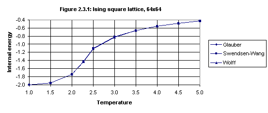
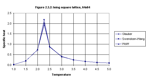
To test the implementation of the Swendsen-Wang and Wolff algorithms the simulations described in Section 2.2 were repeated using these algorithms with lattice size 64x64. These simulation results 7 are given in Figures 2.3.1 and 2.3.2 (which also show the results for the Glauber algorithm for lattice size 64).

Error bars are not shown because the errors were too small. For the Swendsen-Wang algorithm the largest error is 0.0013 at the critical temperature (2.269...) and for the Wolff algorithm it is 0.0015 (also at T_c).

Errors were not estimated in the Swendsen-Wang case. For the Wolff algorithm errors in the measurement of specific heat ranged from a minimum of 0.001 (for T = 1.0) to a maximum of 0.10 (for the critical temperature, T = 2.269...).

The data in Table 2.3.1 (Appendix 5) is summarized below:

Internal energy Temperature 1.00 1.50 2.00 2.27 2.50 3.00 3.50 4.00 4.50 5.00 Glauber -1.997 -1.951 -1.746 -1.431 -1.106 -0.817 -0.661 -0.557 -0.484 -0.428 Sw-Wang -1.997 -1.951 -1.746 -1.424 -1.106 -0.817 -0.659 -0.557 -0.483 -0.429 Wolff -1.997 -1.951 -1.745 -1.434 -1.113 -0.819 -0.661 -0.558 -0.484 -0.429
Specific heat Temperature 1.00 1.50 2.00 2.27 2.50 3.00 3.50 4.00 4.50 5.00 Glauber 0.023 0.197 0.730 2.031 0.860 0.405 0.249 0.171 0.125 0.097 Sw-Wang 0.025 0.197 0.730 2.190 0.881 0.408 0.254 0.176 0.126 0.101 Wolff 0.023 0.197 0.738 1.937 0.885 0.402 0.253 0.169 0.126 0.098

The measurements of internal energy for the three dynamics algorithms are close. Those for specific heat are also close except for the critical temperature (T ≅ 2.269) and T = 2.50. Measurements of specific heat normally vary over a wider range than those for internal energy. These results indicate that the Swendsen-Wang and Wolff algorithms have been implemented correctly, assuming that the Glauber algorithm has been (which seems so on the basis of the results presented in Section 2.2).

The correctness of the implementation of the Swendsen-Wang and the Wolff algorithms is further confirmed by the fact that simulations used to measure the critical temperature and the critical exponent of the magnetization of the Ising model with various lattice types give results confirmed by results published in the literature, as shown in the chapters which follow.

Title page Contents Next: Chapter 3 References

Lattice type:	Square, honeycomb, triangular, cubic, diamond, hypercubic
Lattice size:	Maximum lattice size depends on dimensionality and dynamics algorithm (smaller with cluster algorithms).
Model:	Ising or q-state Potts (for q in the range 2 through 15).
Dynamics:	Metropolis, Glauber, Swendsen-Wang or Wolff.

Temperature(s):	0.0 – 20.0. The temperature can also be specified as "critical", in which case the critical temperature for the type of spin system is used, if known. Multiple temperatures are accepted.
Initial magnetization:	–1.0 through +1.0 (Initial magnetization must be ≥ –1/(q–1) for the q-state Potts model.)
Site concentration:	0.001 – 1.0 (the concentration of occupied sites).
Bond concentration:	0.001 – 1.0 (the concentration of open bonds among pairs of spins located on nearest neighbour sites).

Number of configurations:	1 – 100,000 (but only 1 for a non-diluted lattice)
Number of spin assignments:	1 – 100,000
Number of repetitions:	1 – 500

m(n)	sum of the magnetization (per spin) values
m²(n)	sum of the squares of the magnetization values
m⁴(n)	sum of the fourth powers of the magnetization values
a(n)	sum of the autocorrelation values
e(n)	sum of the actual internal energy values
e²(n)	sum of the squares of the internal energy values