Chapter 3: Critical Temperatures of Pure Ising Spin Models3.1 The Binder Cumulant
Binder and Heerman (1988) define the reduced fourth-order cumulant (a.k.a. the Binder cumulant) for a lattice of linear size L as:
UL = 1 – { M(4)L / [ 3.(M(2)L)2 ] }
where M(2)L is the mean of the squares of the magnetization (with lattice size L) and M(4)L is the mean of the fourth powers of the magnetization (with averages taken over systems at equilibrium at a constant temperature1). They state:
For T > Tc and L >>
ξ [the correlation length2], one can show that UL decreases towards zero as UL ∝ L-d. For T < Tc and L >> ξ ... UL tends to U∞ = 2/3. For L << ξ, on the other hand, UL varies only weakly with temperature and linear dimension ... This behavior of the cumulant makes it very useful for obtaining estimates of Tc ... One may plot UL versus T for various L's and estimate Tc from the common intersection point of these curves." (Binder and Heerman 1988, p.46)Thus suppose we plot UL against T for some lattice of size L. Then for another lattice of size L' > L and any T, if T < Tc we shall obtain UL' > UL, and if T > Tc then UL' < UL. Thus when graphs of UL against T are plotted for a number of lattice sizes they should intersect at a point (or at least their pairwise intersections should be fairly close), the T-value of the intersection point giving an estimate of Tc.
Looked at from another perspective, for a suitable scaling function U
UL = U[(T/Tc - 1).L1/ν]
where ν is the critical exponent of the correlation length (see Binder 1997, p.523).
Thus when T = Tc UL = U(0.L1/ν) = U(0), so at Tc UL has a value independent of L, and so the graphs of UL against T for various L should all pass through a single point at Tc.
The results of the simulations described on the following pages are compared with values for the critical temperatures for the various lattice types given by Fisher (1967, p.671), which were obtained by series expansion. Occasionally a result will be compared with a more recently published result obtained by Monte Carlo studies.
Some simulations were done using Swendsen-Wang dynamics and some using Wolff dynamics.
3.2 Thermal Equilibrium
When measuring the properties of a system it is usual to ensure that the system is in equilibrium. By definition a system is in equilibrium when its bulk properties remain constant (or at least fluctuate closely around a constant mean value) over time, or more exactly, over a time period long enough in the context of the study.
Suppose we boil water, place it in a beaker, and proceed to observe its temperature. Under normal conditions the water will cool and after perhaps an hour it will be at the same temperature as the surrounding air. If the temperature does not change (except for minute fluctuations) over, say, an hour, we can say that the water in the cup has reached thermal equilibrium. Yet if we wait twelve hours we shall probably find that the temperature of the water has changed, because the air temperature has changed, so had the water really reached thermal equilibrium?
Since the properties of spin models do not depend on properties of the systems used to simulate them (such as the temperature of the computer on which the simulation is performed) the question of when thermal equilibrium is attained is somewhat simpler in this case. But basically the idea is the same: A spin system is in thermal equilibrium, with respect to a set of measurable properties (e.g., magnetization and autocorrelation), if those properties have remained constant (or at least have fluctuated closely around a constant mean) over a period of time (or rather, the analogue of time in the model) judged by the investigator to be sufficiently long that no change is likely in the absence of external influences.
Thus if we wish to measure, e.g., the magnetization of a spin system at equilibrium, we must simply allow the system to evolve until the magnetization appears stable. Or rather, the average magnetization, since normally we take averages of measurements at a particular timepoint over many runs.
If we use the Metropolis or the Glauber algorithms to drive the spin system then many timesteps may be required before the magnetization becomes stable, especially if the temperature is close to the critical temperature of the system. As noted in the previous chapter, for this reason dynamics algorithms were developed which cause the spin system to reach equilibrium much more quickly. In this study the Swendsen-Wang and the Wolff algorithms have usually been used, because with these the system typically attains an equilibrium state after less than 40 timesteps.
When measuring some quantity such as the Binder cumulant, it is thus necessary to ascertain first, by experiment, how long it takes for this to stabilize under the algorithm in use, for the lattice sizes and the temperatures at which one wishes to measure the quantity. Then one must decide for how many further timesteps the simulation will be run, since the final measurement of the quantity is the average of the quantity as measured over all timepoints following that at which equilibrium is deemed to have been reached.
For example, suppose we wish to measure the critical temperature, using measurement of the Binder cumulant, of the 2d Ising model on the triangular lattice, and that we plan to use lattice sizes of 20, 30, 40 and 60, temperatures in the range 3.5 through 3.8, and to average over 1000 sample runs in each case. How many timesteps are required for the system to reach equilibrium, and for how long should we run the system further?
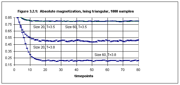
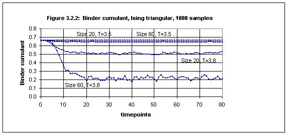
Four simulations were done, using the Swendsen-Wang algorithm, for the four extreme cases: Lattice sizes 20 and 60, and temperatures 3.5 and 3.8.3 The measurements of the absolute magnetization and of the Binder cumulant over timepoints 0 through 80 are shown in Figures 3.2.1 and 3.2.2.4 This shows that for T = 3.5 these quantities stabilize by timepoint 20 and fluctuate hardly at all. For T = 3.8 they appear to fluctuate about a mean from timepoint 30 onwards, and in the case of the Binder cumulant the fluctuations are larger for lattice size 60.
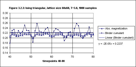
Figure 3.2.3 shows the magnified fluctuations of the Binder cumulant over the time period 40 through 80 (together with the absolute magnetization). The linear trendline for the Binder cumulant data is almost horizontal.
Thus it is reasonable to conclude that with the Swendsen-Wang algorithm the simulations that are intended to be performed are such that the system reaches equilibrium with regard to the absolute magnetization and the Binder cumulant by timepoint 30, and that a time average over timesteps 40 through 80 of the sample averages of the Binder cumulant will provide a satisfactory measurement of this quantity.
To clarify: A simulation actually consists of many "runs" (a.k.a. "samples"), in each of which the spin system is started from some given initial state (e.g., all spins up) and is allowed to evolve over a certain number of timepoints. At each timepoint in a single run measurements are made (e.g., magnetization). The final value for the measurement at each timepoint is the average at that timepoint over all samples.
We normally want measurements to be made when the spin system is in a state of equilibrium. But instead of selecting one timepoint after the system has reached equilibrium we average over a range of timepoints subsequent to the timepoint at which the system is judged to have reached equilibrium. This is called a time average. Thus, e.g., the measured value for the Binder cumulant at a given temperature is actually an average, over a range of timepoints (after equilibrium is reached), of averages of actual measurements made at those timepoints (at that temperature) over many samples.
3.3 The Critical Temperatures of Three Pure 2d Lattices
In this section we shall obtain the critical temperature for the pure 2d Ising model on the square, triangular and honeycomb lattices.
(a) The square lattice
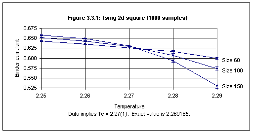
Using Wolff dynamics simulations were performed for the pure square Ising model on six lattices of size 60, 100 and 150, for ten temperatures in the range 2.2 through 2.35 (1000 samples each), and the Binder cumulant was measured. The plots of the Binder cumulant against T, for each size and for five temperatures in the range 2.25 - 2.29, are given in Figure 3.3.1. (The data plotted is taken from Table 3.3.1 of Appendix 5.) At T = 2.27 (close to the critical temperature) the largest error is 0.0022.5
The procedure for arriving at the critical temperature from the data plotted is as follows: For higher temperatures the order of the Binder cumulant graphs (when viewing from top to bottom) is the same as the order of the corresponding lattice sizes, and for lower T the reverse is the case. One looks for the highest T below the intersection point(s) at which the error bars do not overlap, and for the lowest T above the intersection point(s) at which they also do not overlap. Tc is then the mean of these two, and their difference (divided by 2) gives the error bar for Tc.
Thus from the data plotted in Figure 3.3.1 we can conclude that Tc for the square lattice is 2.27(1). Although the precision is not high, this compares well with the actual value of 2.269185 obtained from Onsager's analytical solution (Onsager 1944).
(b) The triangular lattice
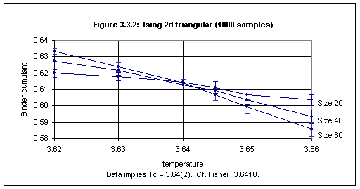
Using Swendsen-Wang dynamics simulations were performed for the pure triangular Ising model on lattices of size 20, 40 and 60, for twelve temperatures in the range 3.5 through 3.8 (in each case 1000 samples were used).
Figure 3.3.2 shows the plots of the Binder cumulant against temperature for each lattice size for six temperatures in the range 3.62 through 3.66 (the data is given in Table 3.3.2 in Appendix 5). By examination of the error bars (as described above) we may conclude that the critical temperature for the triangular lattice is 3.64(2). This compares well with the value given by Fisher (1967, p.671) of 3.6410.
(c) The honeycomb lattice
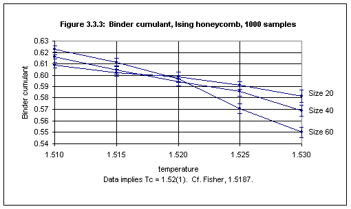
Using Swendsen-Wang dynamics simulations were performed for the pure honeycomb Ising model on lattices of size 20, 40 and 60, for seven temperatures in the range 1.50 through 1.53 (in each case 1000 samples were used).
Figure 3.3.3 shows the plots of the Binder cumulant against temperature for each lattice size for five temperatures in the range 1.51 through 1.53 (the data is taken from Table 3.3.3 in Appendix 5). By examining the error bars in the plots we may conclude that the critical temperature for the triangular lattice is 1.52(1) This compares well with the value given by Fisher (1967, p.671) of 1.5187.
3.4 The Critical Temperatures of Two Pure 3d Lattices
In this section we shall obtain the critical temperatures for the pure 3d Ising model on the cubic and the diamond lattices.
(a) The cubic lattice
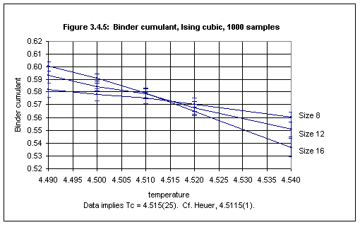
Using Wolff dynamics simulations were performed for the pure cubic Ising model on lattices of size 8, 12 and 16, for ten temperatures in the range 4.4 through 4.6 (in each case 1000 samples were used).
Figure 3.4.5 shows the plots of the Binder cumulant against T for each lattice size for five temperatures in the range 4.49 through 4.54 (the data is given in Table 3.4.5 in Appendix 5).6 From this data we may conclude that the critical temperature for the cubic lattice is 4.515(25). Expressed as Kc = 1/Tc this is 0.2215(12).
This result for Tc compares well with the value given by Fisher (1967, p.671) of 4.5103 (an estimate obtained by high-temperature series expansions). This result also compares well with the value obtained by the Monte Carlo study of Heuer (1993) of 4.5115(1).
Several recent studies using series expansions provide estimates for Kc for the cubic Ising model, as stated in the following table (in order of increasing precision)7:
0.221 67 (2)      Salman and Adler (1991)             Low temperature series expansion
0.221 658 (5)     Salman and Adler (1991)             High temperature series expansion
0.221 665 (5)     Adler (1983)                        Series expansion
0.221 649 (4)     Blöte and Kamieniarz (1994)         Monte Carlo study
0.221 654 4 (10)  Livet (1991)                        Monte Carlo study
0.221 654 6 (10)  Blöte, Luijten and Heringa (1995)   Series expansion
0.221 654 4 (3)   Talapov and Blöte (1996)            Series expansion
Although the value for Kc obtained from this simulation software (namely, 0.2215(12)) is much less precise than the results stated above, the value is accurate; the lack of precision is due to the small number of samples used (1000 for each temperature).
At the critical temperature 1000 samples produce an error of c. 0.0041 in the measurement of the Binder cumulant. Using 6000 samples reduces the error to c. 0.0016, consistent with the fact that reducing the error by a factor of n requires increasing the sample size by n2 (since 0.0041/0.0016 = 2.56 and √6 = 2.45). To reduce the error further to 0.0005 it would be necessary to use c. 60,000 samples, which would require c. 230 hours of computing time on a 330 MHz Intel PC.
(b) The diamond lattice
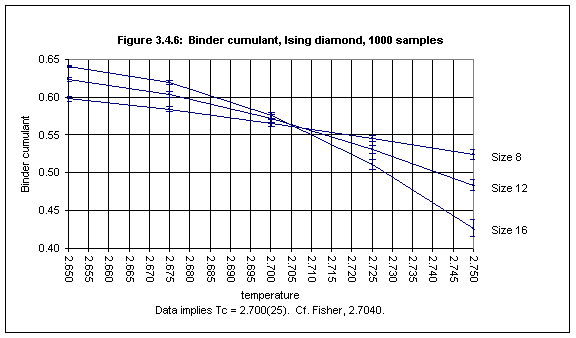
Using Wolff dynamics simulations were performed for the pure diamond Ising model on lattices of size 8, 12 and 16, for seven temperatures in the range 2.6 through 2.8 (in each case 1000 samples were used).
Figure 3.4.6 shows the plots of the Binder cumulant against temperature for each lattice size for five temperatures in the range 2.65 through 2.75 (the data is given in Table 3.4.6 in Appendix 5). We may conclude that the critical temperature for the cubic lattice is 2.700(25). This compares well with the value given by Fisher (1967, p.671) of 2.7040.3.5 The critical temperature of the pure 4d hypercubic lattice
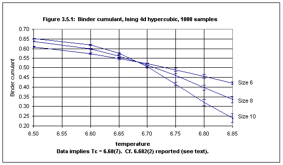
Using Wolff dynamics simulations were performed for the pure 4d hypercubic Ising model on lattices of size 6, 8 and 10, for ten temperatures in the range 6.3 through 7.0 (in each case 1000 samples were used).8
Figure 3.5.1 shows the plots of the Binder cumulant against temperature for each lattice size for seven temperatures in the range 6.50 through 6.85 (the data is given in Table 3.5.1 in Appendix 5). The plots all intersect at 6.68 and we may conclude that the critical temperature for the 4d hypercubic lattice is 6.68(7).
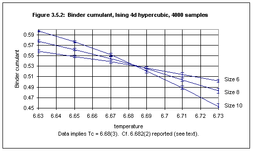
The experiment was repeated with modifications in order to reduce the error in Tc. Simulations were performed for six temperatures in the range 6.63 through 6.73, using 4000 samples. Figure 3.5.2 shows the plots of the Binder cumulant against temperature (the data is given in Table 3.5.2 in Appendix 5).
From this we may conclude that the critical temperature for the Ising 4d hypercubic lattice is 6.68(3).
Gaunt, Sykes and McKenzie (1979) conducted high-temperature series expansion studies of susceptibility in the 4d Ising hypercubic model, and obtained an estimate for 1/vc of 6.732(2), where v = tanh(J/kBT).9 Taking J/kB = 1 this gives an estimate for Tc of 6.682(2).
Thus the Monte Carlo result produced by the simulation software compares well with the more precise estimate of Gaunt et al. obtained from series expansions. To obtain a result with a precision 1/10th of that obtained by the second experiment (i.e.,
±0.003), and thus similar to that of Gaunt's result, it would be necessary to perform the experiment with temperatures in the range 6.680 - 6.684 using 100 x 4,000 = 400,000 samples.10
Title page Contents Next: Chapter 4 References
